In the following set of instructions the following data set will be used for demonstration purposes. It is suggested that you organize your data in a similar format:
| Fin | base | TC1 | TC2 | TC3 | TC4 | TC5 | TC6 | ambient | power (W) |
|---|---|---|---|---|---|---|---|---|---|
| Al_fin_FC | 58.7 | 49.5 | 43.5 | 36.5 | 31.0 | 30.0 | 29.0 | 23.9 | 11.12 |
| Cu_fin_FC | 46.6 | 42.7 | 40.8 | 37.5 | 35.7 | 24.6 | 8.72 | ||
| sqCu_fin_FC | 39.8 | 38.2 | 36.5 | 34.2 | 32.0 | 30.0 | 30.0 | 24.3 | 8.64 |
| SS_fin_FC | 68.0 | 35.6 | 28.6 | 25.3 | 24.5 | 24.5 | 24.5 | 24.0 | 6.37 |
| Fin | base | 1 | 2 | 3 | 4 | 5 | 6 |
|---|---|---|---|---|---|---|---|
| Al_fin_FC | 1.87 | 2.80 | 3.11 | 3.00 | 2.37 | 2.25 | 1.98 |
| Cu_fin_FC | 1.85 | 2.95 | 3.27 | 3.21 | 2.82 | ||
| sqCu_fin_FC | 1.88 | 2.65 | 3.20 | 3.15 | 2.78 | 2.58 | 2.14 |
| SS_fin_FC | 1.56 | 2.63 | 3.08 | 3.15 | 2.95 | 2.64 | 2.24 |
| Fin | base | TC1 | TC2 | TC3 | TC4 | TC5 | TC6 | ambient | power (W) |
|---|---|---|---|---|---|---|---|---|---|
| Al_fin_NC | 90.7 | 83.5 | 77.9 | 70.4 | 63.1 | 60.9 | 59.0 | 24.2 | 11.12 |
| Cu_fin_NC | 80.6 | 78.3 | 77.1 | 74.3 | 72.9 | 24.7 | 8.72 | ||
| sqCu_fin_NC | 67.7 | 66.3 | 65.3 | 63.0 | 60.4 | 58.4 | 58.4 | 24.5 | 8.64 |
| SS_fin_NC | 86.5 | 58.2 | 45.5 | 33.2 | 26.6 | 25.0 | 25.0 | 24.1 | 6.37 |
The input files which make use of the EFCcyl and EFCdiamond forced convection correlation conductors are:
| Fin | Forced Convection |
|---|---|
| Aluminum, 11.22” | Al_fin_FC.inp |
| Round Copper, 6.77” | Cu_fin_FC.inp |
| Square Copper, 11.22” | sqCu_fin_FC.inp |
| Stainless Steel, 11.22” | SS_fin_FC.inp |
For each fin, open the input file in an editor and set the boundary temperatures Tc and Tr to ambient and base to base. Here is the Al_fin_FC.inp file in an editor, with the boundary condition values set to the values in the table shown above:
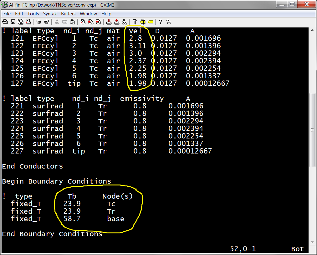
You should verify that the flow velocities are set to the correct values. If not, edit the file and set them to the desired value. Make sure to save the changes you have made.
Now run the model with TNSolver in MATLAB/Octave:
>> tnsolver('Al_fin_FC');

**********************************************************
*                                                        *
*          TNSolver - A Thermal Network Solver           *
*                                                        *
*             Version 0.9.2, August 9, 2017              *
*                                                        *
**********************************************************

Reading the input file: Al_fin_FC.inp

Initializing the thermal network model ...

Starting solution of a steady thermal network model ...

     Nonlinear Solve
  Iteration    Residual
  ---------  ------------
        1     54.6816
        2     0.337734
        3     0.000168644
        4     6.92131e-08
        5     3.05718e-11

Results have been written to: Al_fin_FC.out

Node results have been written to: Al_fin_FC_nd.csv

Conductor results have been written to: Al_fin_FC_cond.csv

All done ...

>>
|
Now open the output file Al_fin_FC.out in your favorite editor in order to find the heat transfer coefficient data from the correlations:
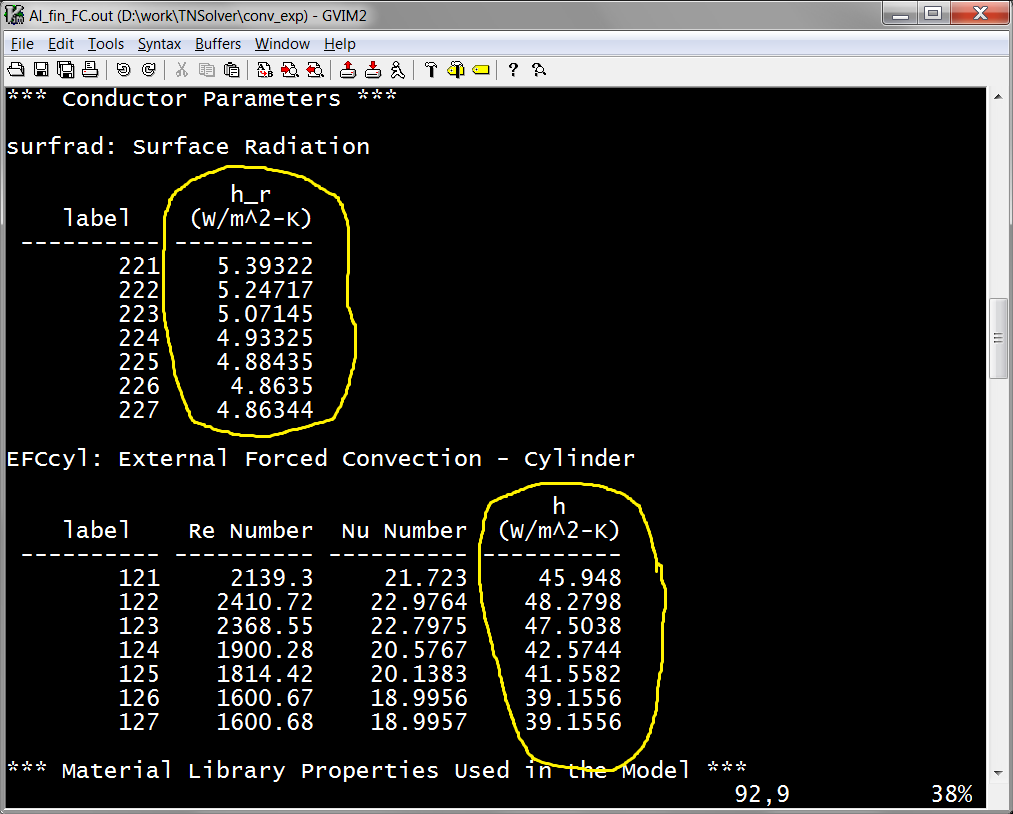
Repeat this process for each of the four fins. These are the heat transfer coefficients, using the forced convection correlation, that you want to compare to your h from the least squares analysis with the analytical fin experiment.
| Fin | base | TC1 | TC2 | TC3 | TC4 | TC5 | TC6 | ambient | power (W) |
|---|---|---|---|---|---|---|---|---|---|
| Al_fin_NC | 90.7 | 83.5 | 77.9 | 70.4 | 63.1 | 60.9 | 59.0 | 24.2 | 11.12 |
| Cu_fin_NC | 80.6 | 78.3 | 77.1 | 74.3 | 72.9 | 24.7 | 8.72 | ||
| sqCu_fin_NC | 67.7 | 66.3 | 65.3 | 63.0 | 60.4 | 58.4 | 58.4 | 24.5 | 8.64 |
| SS_fin_NC | 86.5 | 58.2 | 45.5 | 33.2 | 26.6 | 25.0 | 25.0 | 24.1 | 6.37 |
The input files which make use of the ENChcyl natural convection correlation conductors are:
| Fin | Natural Convection |
|---|---|
| Aluminum, 11.22” | Al_fin_NC.inp |
| Round Copper, 6.77” | Cu_fin_NC.inp |
| Square Copper, 11.22” | sqCu_fin_NC.inp |
| Stainless Steel, 11.22” | SS_fin_NC.inp |
For each fin, open the input file in an editor and set the boundary temperatures Tc and Tr to ambient and base to base. Here is the Cu_fin_NC.inp file in an editor, with the boundary condition values set to the values in the table shown above:
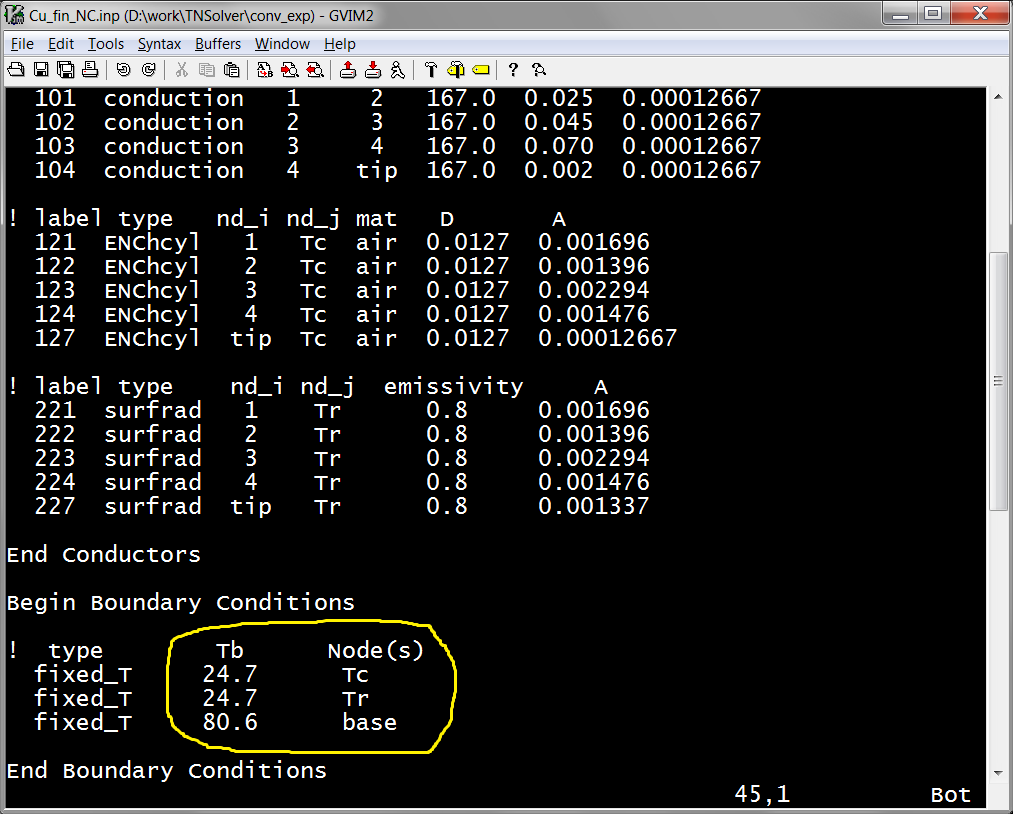
Make sure to save the changes you have made.
Now run the model with TNSolver in MATLAB/Octave:
>> tnsolver('Cu_fin_NC');

**********************************************************
*                                                        *
*          TNSolver - A Thermal Network Solver           *
*                                                        *
*             Version 0.9.2, August 9, 2017              *
*                                                        *
**********************************************************

Reading the input file: Cu_fin_NC.inp

Initializing the thermal network model ...

Starting solution of a steady thermal network model ...

     Nonlinear Solve
  Iteration    Residual
  ---------  ------------
        1     58.3599
        2     1.20591
        3     0.00962502
        4     9.06156e-05
        5     9.66255e-07
        6     1.03889e-08
        7     1.11883e-10

Results have been written to: Cu_fin_NC.out

Node results have been written to: Cu_fin_NC_nd.csv

Conductor results have been written to: Cu_fin_NC_cond.csv

All done ...

>>
|
Now open the output file Cu_fin_NC.out in your favorite editor in order to find the heat transfer coefficient data from the correlations:
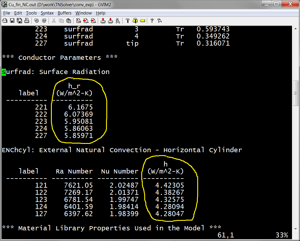
Repeat this process for each of the four fins. These are the heat transfer coefficients, using the natural convection correlation, that you want to compare to your h from the least squares analysis with the analytical fin experiment.
| Fin | base | TC1 | TC2 | TC3 | TC4 | TC5 | TC6 | ambient | power (W) |
|---|---|---|---|---|---|---|---|---|---|
| Al_fin_FC | 58.7 | 49.5 | 43.5 | 36.5 | 31.0 | 30.0 | 29.0 | 23.9 | 11.12 |
| Cu_fin_FC | 46.6 | 42.7 | 40.8 | 37.5 | 35.7 | 24.6 | 8.72 | ||
| sqCu_fin_FC | 39.8 | 38.2 | 36.5 | 34.2 | 32.0 | 30.0 | 30.0 | 24.3 | 8.64 |
| SS_fin_FC | 68.0 | 35.6 | 28.6 | 25.3 | 24.5 | 24.5 | 24.5 | 24.0 | 6.37 |
For each of the experimental data sets, find the best emissivity that fits your experimental data, using the correlations for the heat transfer coefficient.
| Fin | Forced Convection |
|---|---|
| Aluminum, 11.22” | Al_fin_FC.inp |
| Round Copper, 6.77” | Cu_fin_FC.inp |
| Square Copper, 11.22” | sqCu_fin_FC.inp |
| Stainless Steel, 11.22” | SS_fin_FC.inp |
For each fin, open the input file in an editor and set the boundary temperatures Tc and Tr to ambient and base to base. Here is the Al_fin_FC.inp file in an editor, with the boundary condition values set to the values in the table shown above:
Note that if you did the first step above, 1) Forced Convection Correlation Results, then you have already set the correct boundary conditions in the file.
You should verify that the flow velocities are set to the correct values. If not, edit the file and set them to the desired value. Make sure to save the changes you have made.
Now run the model with ls_fin_emiss in MATLAB/Octave:
>>emiss = linspace(0.01,1.0,20);
>>expT = [ 49.5 43.5 36.5 31.0 30.0 29.0 ];
>>beste = ls_fin_emiss('Al_fin_FC', expT, emiss)

**********************************************************
*                                                        *
*          TNSolver - A Thermal Network Solver           *
*                                                        *
*  Modified Version for Least Squares Fit of Emissivity  *
*                                                        *
*             Version 0.9.2, August 9, 2017              *
*                                                        *
**********************************************************

Reading the input file: Al_fin_FC.inp

Initializing the thermal network model ...

Starting solution of a steady thermal network model ...

     Nonlinear Solve
  Iteration    Residual
  ---------  ------------
        1     53.5385
        2     0.00506803
        3     1.75073e-06
        4     8.28495e-10

***** intermediate screen output deleted *****

     Nonlinear Solve
  Iteration    Residual
  ---------  ------------
        1     0.0449049
        2     1.81694e-05
        3     7.53064e-09

Results have been written to: Al_fin_FC.out

Node results have been written to: Al_fin_FC_nd.csv

Conductor results have been written to: Al_fin_FC_cond.csv

All done ...


beste =

    0.4789
|
The best fit emissivity, beste, is printed to the screen at the end of the run. In addition, a plot of the residual vs. emissivity is provided. Make sure that you actually found the minimum with your chosen range:
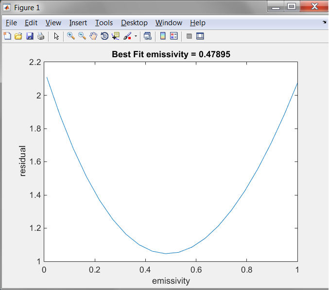
Repeat this process for all four forced convection experimental data sets and record the best fit emissivity for each one. How does the emissivity compare to the table value (see Table A.8)? Is the emissivity within physical bounds (0 < ε < 1)?
| Fin | base | TC1 | TC2 | TC3 | TC4 | TC5 | TC6 | ambient | power (W) |
|---|---|---|---|---|---|---|---|---|---|
| Al_fin_NC | 90.7 | 83.5 | 77.9 | 70.4 | 63.1 | 60.9 | 59.0 | 24.2 | 11.12 |
| Cu_fin_NC | 80.6 | 78.3 | 77.1 | 74.3 | 72.9 | 24.7 | 8.72 | ||
| sqCu_fin_NC | 67.7 | 66.3 | 65.3 | 63.0 | 60.4 | 58.4 | 58.4 | 24.5 | 8.64 |
| SS_fin_NC | 86.5 | 58.2 | 45.5 | 33.2 | 26.6 | 25.0 | 25.0 | 24.1 | 6.37 |
For each of the experimental data sets, find the best emissivity that fits your experimental data, using the correlations for the heat transfer coefficient.
| Fin | Natural Convection |
|---|---|
| Aluminum, 11.22” | Al_fin_NC.inp |
| Round Copper, 6.77” | Cu_fin_NC.inp |
| Square Copper, 11.22” | sqCu_fin_NC.inp |
| Stainless Steel, 11.22” | SS_fin_NC.inp |
For each fin, open the input file in an editor and set the boundary temperatures Tc and Tr to ambient and base to base. Here is the Cu_fin_NC.inp file in an editor, with the boundary condition values set to the values in the table shown above:
Note that if you did the second step above, 1) Natural Convection Correlation Results, then you have already set the correct boundary conditions in the file.
Make sure to save the changes you have made.
Now run the model with ls_fin_emiss in MATLAB/Octave:
>>emiss = linspace(0.01,1.0,20);
>>expT = [ 78.3 77.1 74.3 72.9 ];
>>beste = ls_fin_emiss('Cu_fin_NC', expT, emiss)

**********************************************************
*                                                        *
*          TNSolver - A Thermal Network Solver           *
*                                                        *
*  Modified Version for Least Squares Fit of Emissivity  *
*                                                        *
*             Version 0.9.2, August 9, 2017              *
*                                                        *
**********************************************************


Reading the input file: Cu_fin_NC.inp

Initializing the thermal network model ...

Starting solution of a steady thermal network model ...

     Nonlinear Solve
  Iteration    Residual
  ---------  ------------
        1     57.5138
        2     0.215554
        3     0.00248576
        4     3.29208e-05
        5     4.446e-07
        6     6.022e-09

***** intermediate screen output deleted *****

     Nonlinear Solve
  Iteration    Residual
  ---------  ------------
        1     0.139323
        2     0.00124206
        3     1.24777e-05
        4     1.27279e-07
        5     1.30168e-09

Results have been written to: Cu_fin_NC.out

Node results have been written to: Cu_fin_NC_nd.csv

Conductor results have been written to: Cu_fin_NC_cond.csv

All done ...


beste =

    0.0621
|
The best fit emissivity, beste, is printed to the screen at the end of the run. In addition, a plot of the residual vs. emissivity is provided. Make sure that you actually found the minimum with your chosen range:
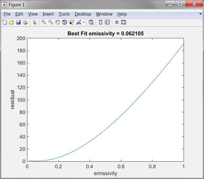
Repeat this process for all four natural convection experimental data sets and record the best fit emissivity for each one. How does the emissivity compare to the table value (see Table A.8)? Is the emissivity within physical bounds (0 < ε < 1)?
| Fin | base | TC1 | TC2 | TC3 | TC4 | TC5 | TC6 | ambient | power (W) |
|---|---|---|---|---|---|---|---|---|---|
| Al_fin_C | 58.7 | 49.5 | 43.5 | 36.5 | 31.0 | 30.0 | 29.0 | 23.9 | 11.12 |
| Cu_fin_C | 46.6 | 42.7 | 40.8 | 37.5 | 35.7 | 24.6 | 8.72 | ||
| sqCu_fin_C | 39.8 | 38.2 | 36.5 | 34.2 | 32.0 | 30.0 | 30.0 | 24.3 | 8.64 |
| SS_fin_C | 68.0 | 35.6 | 28.6 | 25.3 | 24.5 | 24.5 | 24.5 | 24.0 | 6.37 |
For each of the experimental data sets, find the best fit heat transfer coefficient that fits your experimental data, using the emissivity you found in step 3) Using a Least-Squares Residual Approach, Find the Emissivity, ε, for the Forced Convection Experimental Data. The input files you will be using are the convection input files:
| Fin | Convection |
|---|---|
| Aluminum, 11.22” | Al_fin_C.inp |
| Round Copper, 6.77” | Cu_fin_C.inp |
| Square Copper, 11.22” | sqCu_fin_C.inp |
| Stainless Steel, 11.22” | SS_fin_C.inp |
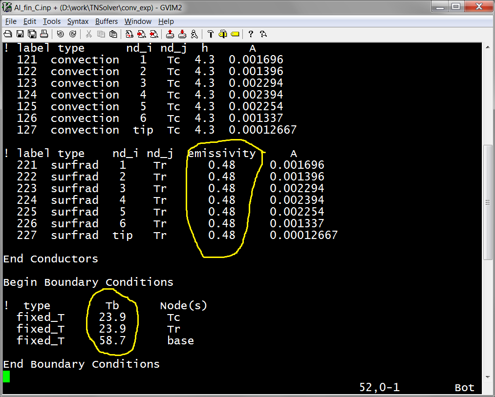
For each fin, open the input file in an editor and set the boundary temperatures Tc and Tr to ambient and base to base. Set the emissivity value on the surfrad conductors to the value you found in step 3). Here is the Al_fin_C.inp file in an editor, with the boundary condition values set to the values in the table shown above, as well as the emissivity:
Now run the model with ls_fin_h in MATLAB/Octave:
>> h = linspace(30,60,20);
>> expT = [ 49.5 43.5 36.5 31.0 30.0 29.0 ];
>> besth = ls_fin_h('Al_fin_C',expT,h)

**********************************************************
*                                                        *
*          TNSolver - A Thermal Network Solver           *
*                                                        *
*       Modified Version for Least Squares Fit of h      *
*                                                        *
*             Version 0.9.2, August 9, 2017              *
*                                                        *
**********************************************************

Reading the input file: Al_fin_C.inp

Initializing the thermal network model ...

Starting solution of a steady thermal network model ...

     Nonlinear Solve
  Iteration    Residual
  ---------  ------------
        1     50.3294
        2     0.239163
        3     1.9008e-05
        4     8.43839e-13

***** intermediate screen output deleted *****

     Nonlinear Solve
  Iteration    Residual
  ---------  ------------
        1     0.190658
        2     3.79629e-06
        3     4.88472e-13

Results have been written to: Al_fin_C.out

Node results have been written to: Al_fin_C_nd.csv

Conductor results have been written to: Al_fin_C_cond.csv

All done ...


besth =

   44.2105
|
The best fit convection coefficient, besth, is printed to the screen at the end of the run. In addition, a plot of the residual vs. h is provided. Make sure that you actually found the minimum with your chosen range:
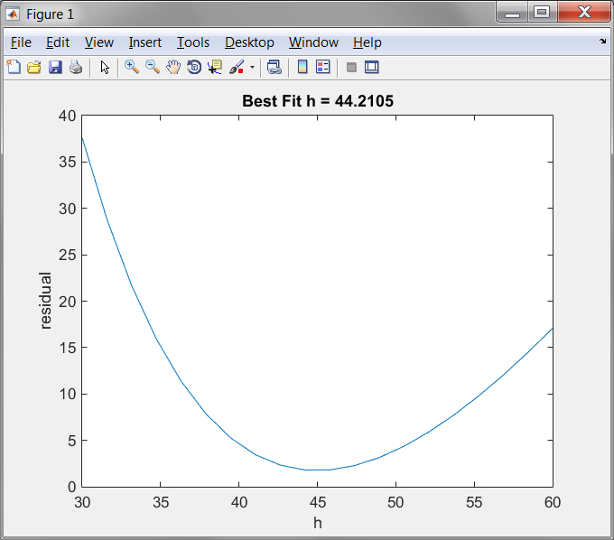
Repeat this process for all four forced convection experimental data sets and record the best fit h for each one.
| Fin | base | TC1 | TC2 | TC3 | TC4 | TC5 | TC6 | ambient | power (W) |
|---|---|---|---|---|---|---|---|---|---|
| Al_fin_C | 90.7 | 83.5 | 77.9 | 70.4 | 63.1 | 60.9 | 59.0 | 24.2 | 11.12 |
| Cu_fin_C | 80.6 | 78.3 | 77.1 | 74.3 | 72.9 | 24.7 | 8.72 | ||
| sqCu_fin_C | 67.7 | 66.3 | 65.3 | 63.0 | 60.4 | 58.4 | 58.4 | 24.5 | 8.64 |
| SS_fin_C | 86.5 | 58.2 | 45.5 | 33.2 | 26.6 | 25.0 | 25.0 | 24.1 | 6.37 |
For each of the natural convection experimental data sets, find the best fit heat transfer coefficient that fits your experimental data, using the emissivity you found in step 4) Using a Least-Squares Residual Approach, Find the Emissivity, ε, for the Natural Convection Experimental Data. The input files you will be using are the convection input files:
| Fin | Convection |
|---|---|
| Aluminum, 11.22” | Al_fin_C.inp |
| Round Copper, 6.77” | Cu_fin_C.inp |
| Square Copper, 11.22” | sqCu_fin_C.inp |
| Stainless Steel, 11.22” | SS_fin_C.inp |
For each fin, open the input file in an editor and set the boundary temperatures Tc and Tr to ambient and base to base. Set the emissivity value on the surfrad conductors to the value you found in step 3). Here is the Cu_fin_C.inp file in an editor, with the boundary condition values set to the values in the table shown above, as well as the emissivity:
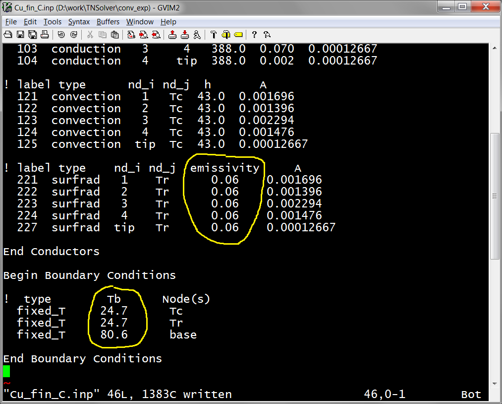
Now run the model with ls_fin_h in MATLAB/Octave:
>> h = linspace(2,12,20);
>> expT = [ 78.3 77.1 74.3 72.9 ];
>> besth = ls_fin_h('Cu_fin_C',expT,h)
**********************************************************
* *
* TNSolver - A Thermal Network Solver *
* *
* Modified Version for Least Squares Fit of h *
* *
* Version 0.9.2, August 9, 2017 *
* *
**********************************************************
Reading the input file: Cu_fin_C.inp
Initializing the thermal network model ...
Starting solution of a steady thermal network model ...
Nonlinear Solve
Iteration Residual
--------- ------------
1 132.444
2 0.081304
3 1.98662e-07
4 1.81884e-12
***** intermediate screen output deleted *****
Nonlinear Solve
Iteration Residual
--------- ------------
1 0.186277
2 8.20996e-07
3 3.5291e-13
Results have been written to: Cu_fin_C.out
Node results have been written to: Cu_fin_C_nd.csv
Conductor results have been written to: Cu_fin_C_cond.csv
All done ...
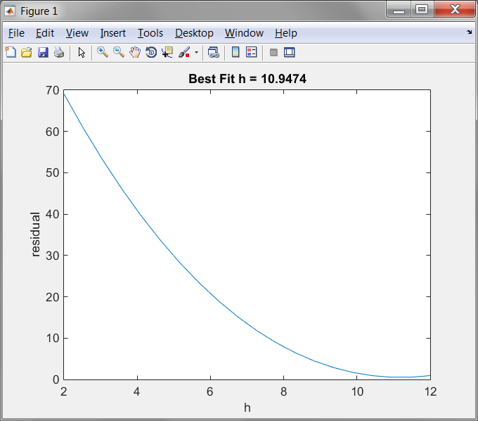
besth =
10.9474
|
The best fit convection coefficient, besth, is printed to the screen at the end of the run. In addition, a plot of the residual vs. h is provided. Make sure that you actually found the minimum with your chosen range:
Repeat this process for all four natural convection experimental data sets and record the best fit h for each one.